A Sharpe ratio tells you how large a strategy's risk-adjusted return was over a sample. It does not tell you whether that return was earned month after month or in 3 good years that happened to fall inside the window. 2 strategies with the same Sharpe ratio over the same 40 years can have very different histories, and the number is silent about it. The Robustness score we added in August asks a different question, whether the Sharpe ratio survives the number of strategies we tried, and it is also silent on this one.
In early September the Stability column went live on the leaderboard, after Roman Rubsamen, who runs the Portfolio Optimizer service and blog, pointed us to a working paper by Mario Bajo Traver and Alejandro Rodriguez Dominguez that proposes a clean answer: the Sharpe Stability Ratio. This post is longer and more technical than usual because the statistic deserves it, because we ran it across our entire catalog rather than a handful of examples, and because the results changed how we read our own leaderboard. That catalog-wide run is now published as a working paper on SSRN, The Sharpe Stability Ratio in Tactical and Static Asset Allocation Backtests: Evidence from 173 Published Strategy Variants (23 pages, DOI 10.2139/ssrn.7441662), together with a public replication archive holding the code, the result tables and the fixture that produced every number below. What follows are the parts that matter for choosing a strategy.
What the ratio measures
Take a strategy's monthly returns and compute its Sharpe ratio over every 36-month window, sliding one month at a time. That rolling series is the object of interest. Its mean says how good the strategy was on average; its dispersion says how much the risk-adjusted return swung from one 3-year stretch to the next. The Sharpe Stability Ratio is the 1st divided by the 2nd:
SSR = mean of the rolling 36-month Sharpe ratio / long-run standard deviation of that rolling series
The subtlety is in the denominator. Overlapping windows share 35 of their 36 months, so consecutive rolling Sharpe ratios are almost identical by construction and the ordinary standard deviation of the series understates its true variability by a factor of 4 or 5. Bajo Traver and Rodriguez Dominguez fix this with the Newey-West long-run variance with a triangular kernel, which adds the autocovariances of the series at lags up to a bandwidth with declining weights. We fix that bandwidth at 35 lags, the full extent of the overlap, so that every strategy is measured with the same estimator. The paper lets an automatic bandwidth rule choose it (15 lags in its sample) and shows that the choice moves the level of the ratio by a third while leaving the ranking almost untouched (rank correlation 0.98). Our own check agrees: across 4 bandwidths the median value runs from 0.41 to 0.87 and the rank correlations with our baseline stay between 0.94 and 0.99. Compare orderings across implementations, never levels.
The benchmark Sharpe ratio is 0, so the ratio reads as "how consistently did the rolling Sharpe stay above 0". A value near 0 means the strategy's Sharpe ratio swung between positive and negative stretches. Around one is steady across regimes. Values far above one deserve suspicion rather than applause: in Roman Rubsamen's Portfolio Optimizer write-up that brought the paper to our attention, Bernard Madoff's feeder fund scored 1.55 over 20 years. We require 10 years of monthly history and show n/a below it, which is why the 5-year leaderboard view has no Stability values at all.
The catalog it was run on
The study covers the 177 strategy variants on our public leaderboard as of 5 September 2026. 3 variants of one strategy are set aside pending a data restatement and one has less than the 10 years of history the statistic needs, which leaves 173. The figures below use completed months through August 2026; the live Stability column keeps the current month, so it differs from them in the 3rd decimal. Every variant is simulated by the same engine on the same adjusted prices, with 10 basis points of one-way cost and execution the session after a signal, and the statistic is computed on exactly the month-end series that defines our published Sharpe and Sortino ratios. The histories are long: 486 months at the median, 1,274 at the longest, with 144 of the 173 starting before 1990 and 34 before 1980. The catalog holds 142 tactical variants (momentum, trend, breadth, volatility and macro rules) and 31 static allocations, from the classic 60/40 to the Golden Butterfly; 52 variants use leverage.
We computed everything twice, once in a standalone script written from the paper's definitions and once in the production service that now feeds the leaderboard, written separately from a specification. The 2 agree to 15 decimals. The same script reproduces the leaderboard's Robustness scores to 4 decimals, so the 2 columns are computed on the same series.
What the numbers say
Across the 173 variants the full-history Stability runs from 0.15 to 0.98 with a median of 0.44. 55 variants sit at or above 0.5 and 12 at or above 0.7. The S&P 500 (through the Vanguard 500 fund, since 1976) scores 0.30 and a monthly-rebalanced 60/40 blend 0.33, the 2 in the bottom 1/4 of the catalog.
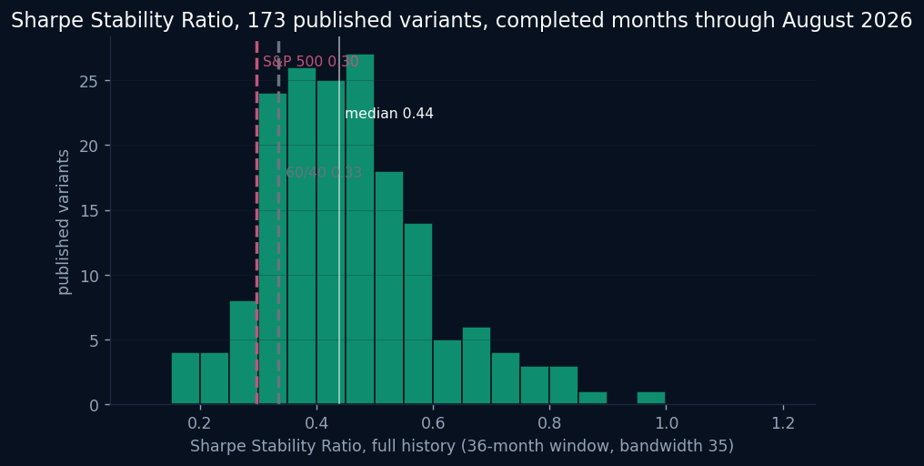
The first thing the column does is resolve the top of the Robustness ranking. 88 of the 173 variants carry a Robustness score of 1.00 at 2 decimals, because a long history makes almost any decent Sharpe ratio statistically credible. Those 88 are spread across the whole Stability range. Table 1 puts the 2 scores side by side: 146 variants clear the Robustness threshold of 0.90, but only 54 of them also clear a Stability of 0.5. 92 strategies are credible without being steady. For a catalog of long backtests, credibility is the easy bar and consistency is the discriminating one.
| Stability at or above 0.5 | Stability below 0.5 | |
|---|---|---|
| Robustness at or above 0.90 | 54 | 92 |
| Robustness below 0.90 | 1 | 26 |
Table 1. The 173 published variants classified by Robustness (Deflated Sharpe Ratio) and full-history Stability.
The second thing it does is disagree with the Sharpe ratio, but not randomly. The rank correlation between Stability and the Sharpe ratio is 0.67: the 2 agree on the broad picture and disagree on a third of the ordering. Stability is only weakly related to the growth rate (rank correlation 0.20) and moderately to the depth of the worst drawdown (0.49: shallower drawdowns, steadier Sharpe). Hybrid Asset Allocation is the clearest case. It has one of the highest Sharpe ratios in the catalog at 1.49, its rolling Sharpe never went negative in 595 rolling windows, and its Stability is 0.52, because the level of that rolling Sharpe swung widely across 5 decades and the long-run dispersion of a 52-year series is large. Since 2000 it scores 0.88. Global Equities Momentum, with a Sharpe ratio of 0.99, scores 0.39.
| Strategy | Since | Sharpe | Robustness | Stability, full | Since 2000 | Since 2008 |
|---|---|---|---|---|---|---|
| Momentum-Correlation Triplet | 1987 | 1.24 | 1.000 | 0.98 | 0.91 | 0.78 |
| Lethargic Asset Allocation (LAA) | 1986 | 1.20 | 1.000 | 0.63 | 0.70 | 0.77 |
| Bold Asset Allocation (BAA-G12) | 1986 | 1.26 | 1.000 | 0.57 | 0.51 | 0.50 |
| Hybrid Asset Allocation (HAA) | 1974 | 1.49 | 1.000 | 0.52 | 0.88 | 0.89 |
| Golden Butterfly | 1988 | 1.14 | 0.999 | 0.50 | 0.53 | 0.63 |
| Defensive Asset Allocation (DAA-G12) | 1986 | 1.32 | 1.000 | 0.49 | 0.48 | 0.48 |
| Global Tactical Asset Allocation (GTAA-5) | 1986 | 1.20 | 1.000 | 0.45 | 0.41 | 0.88 |
| All Weather | 1972 | 0.98 | 0.999 | 0.45 | 0.41 | 0.38 |
| Global Equities Momentum (GEM) | 1986 | 0.99 | 0.994 | 0.39 | 0.38 | 0.52 |
| Classic 60/40 | 1923 | 0.73 | 0.945 | 0.29 | 0.37 | 0.63 |
| S&P 500 (VFINX) | 1976 | 0.75 | n/a | 0.30 | 0.29 | 0.74 |
Table 2. Widely followed strategies and the S&P 500 on 3 windows. Sharpe is the full-history monthly-mean ratio; Robustness is the published Deflated Sharpe Ratio.
The third thing it does is rank strategy families in a way the Sharpe ratio does not. Tactical variants have a median Stability of 0.45 against 0.37 for static allocations. Monthly-rebalanced strategies are the steadiest frequency group at 0.47; daily strategies score 0.37 and annually rebalanced allocations 0.34. Leveraged variants are slightly less steady than unleveraged ones (0.41 against 0.45), and by our risk categories the conservative group scores 0.50, the moderate group 0.47 and the aggressive group 0.38. Aggressive strategies buy their higher average Sharpe ratio with more swing around it.
Stability belongs to the window, not to the strategy
This is the result that changed how we read the column. Everything above was computed on the full history. Compute the same statistic since January 2000, a window that contains 2 bear markets, and the picture holds: the S&P 500 scores 0.29 and 153 of the 166 variants with data over that window beat it. Compute it since January 2008, one bear market followed by a 15-year expansion, and the picture inverts: the S&P 500 scores 0.74, the Nasdaq 100 0.88, and only 55 of 172 variants beat the S&P 500. The rank correlation between the 2 windows is 0.53.
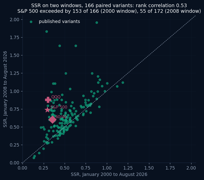
Splitting the calendar into decades makes the point brutally. Inside each of 4 subperiods (before 2000, the 2000s, the 2010s, and 2020 to now) we recomputed the ratio for every variant with at least 6 years of data. The median across the catalog was 0.66, 0.82, 1.02 and 0.82. The cross-sectional rank correlation between adjacent decades was -0.04, -0.43 and 0.08. Between the 2000s and the 2010s it is strongly negative: the strategies that were steadiest through the dot-com and financial crises were the least steady through the expansion that followed, while the S&P 500 went from 0.15 to 1.63 and long Treasuries from the steadiest series of the 2000s (3.38) to a negative ratio in the 2020s. Bajo Traver and Rodriguez Dominguez report an average subperiod rank correlation of 0.31 for hedge fund indices and call the ratio "inherently conditional on the prevailing market regime". For rules-based allocation strategies, whose defensive legs are themselves regime bets, the dependence looks stronger still, although the samples and estimators differ.
| Before 2000 | 2000 to 2009 | 2010 to 2019 | 2020 to Aug 2026 | |
|---|---|---|---|---|
| Median Stability, published variants | 0.66 | 0.82 | 1.02 | 0.82 |
| S&P 500 (VFINX) | 0.40 | 0.15 | 1.63 | 0.81 |
| 60/40 (VFINX/VBMFX) | 0.63 | 0.23 | 1.60 | 0.59 |
| Long Treasuries (TLT) | n/a | 3.38 | 0.80 | -0.47 |
| Rank correlation with the previous decade | -0.04 | -0.43 | 0.08 |
Table 3. Stability inside 4 subperiods (6-year minimum, so levels are inflated relative to the full-history values and only the ordering should be read), and the rank correlation of the cross-section between adjacent subperiods.
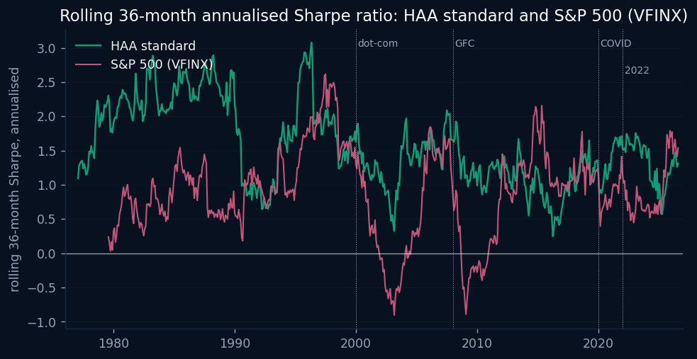
This is why the leaderboard recomputes Stability for every period you select rather than showing one number, and why a strategy page shows the full-history value with that qualifier. A window dominated by a long bull market makes buy-and-hold look steady, and it is not wrong to say so; it is wrong to read it as a property the strategy will carry into the next window. Try several start dates before drawing a conclusion. The statistic describes what happened. It does not forecast.
Trading more does not cost consistency
A natural guess is that stability rewards patience and that strategies that trade less should have smoother risk-adjusted returns. The catalog says the opposite. The rank correlation between annual turnover and Stability is +0.31. Split the variants into turnover terciles and the lowest tercile (up to 1.4 times the portfolio per year, mostly static allocations and slow trend rules) has a median Stability of 0.41, the middle tercile 0.41, and the highest tercile (3 to 15 times per year, all of it tactical) 0.50. The median Sharpe ratio is nearly identical across the 3 (0.98, 1.00, 1.00), so the difference is in consistency, not level. 2 cautions. The terciles differ in composition, since every static allocation sits in the lowest one, and within tactical variants alone the rank correlation drops to 0.23; this is an association, not a measured effect of trading. The mechanism we suspect, and have not tested, is Figure 3 again: a static allocation carries its full equity exposure into every bear market and its rolling Sharpe ratio is driven below 0 each time, while a monthly rotation with a defensive leg spends those months elsewhere.
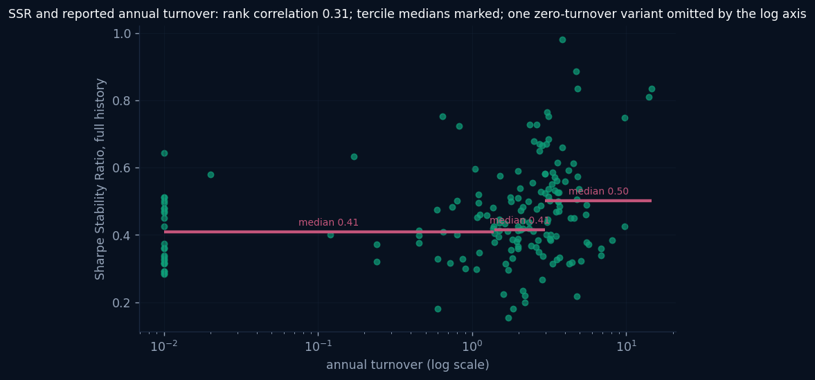
A word on what turnover means here. The engine trades to a signal's target weights on the session after the signal and then holds the positions, letting the weights drift, until the next signal; the annual turnover on the leaderboard is the fraction of the portfolio traded at those points, summed over a year. 1-asset regimes trade only when their signal flips, static allocations only on their rebalancing schedule, and monthly rotations at most 1 time a month, which is why the terciles above line up so cleanly with strategy type.
How sure are the numbers
The paper recommends a moving block bootstrap for inference, because overlapping windows make the usual asymptotics unreliable. We resampled each variant's monthly returns in contiguous 36-month blocks, 2,000 times, and recomputed the ratio on every replicate. Every one of the 173 intervals excludes 0, so temporal stability in this catalog is not sampling noise. 0 variants reject the hypothesis that its true ratio is at or below 0.5 at the 5 percent level, and the median 95 percent interval is 0.45 wide. The same pattern holds in the paper's hedge fund sample. The point estimates order the strategies; the ordering between neighbours is not statistically sharp. Read the column as a ranking aid, not a certificate. Every interval, and the script that produced it, is in the replication archive.
2 more robustness checks, briefly. Rolling windows of 24, 36, 48 and 60 months produce rank correlations of 0.96 to 0.98 between adjacent lengths, with levels rising as the window lengthens. And the autocorrelation-aware Sharpe ratio variance that López de Prado, Lipton and Zoonekynd published this year, which Roman also asked us about, changes nothing for the Robustness score: our returns are monthly, their lag-one autocorrelation has a median of -0.03 across the catalog, and recomputing every Robustness score with the new variance moves 0 of them by more than 0.021.
What to do with it
Use Stability to separate strategies whose Robustness scores tie, which on this leaderboard is most of them. Use it on the period you actually care about, and on 2 or 3 others, and treat a strategy whose ranking survives the change of window as more trustworthy than one that does not. Do not use it to pick the highest number: above about one, ask what the strategy is doing rather than admire it, and remember that a static equity allocation will carry a high value out of any window that ends in a long bull market. And keep the Sharpe ratio: the 2 disagree on a third of the ordering, and the disagreement is the information.
References: this post summarises our working paper The Sharpe Stability Ratio in Tactical and Static Asset Allocation Backtests: Evidence from 173 Published Strategy Variants (2026), SSRN 7441662, DOI 10.2139/ssrn.7441662, with code and result tables at github.com/lbonherbe/sharpe-stability-ratio-taa. It builds on Bajo Traver, M. and Rodriguez Dominguez, A. (2026), The Sharpe Stability Ratio: Temporal Consistency of Risk-Adjusted Performance, SSRN 6344658; López de Prado, M., Lipton, A. and Zoonekynd, V. (2026), How to Use the Sharpe Ratio, ADIA Lab Research Paper Series No. 19; Bailey, D. H. and López de Prado, M. (2014), The Deflated Sharpe Ratio, Journal of Portfolio Management 40(5); Newey, W. K. and West, K. D. (1987), Econometrica 55(3); Rubsamen, R. (2026), The Sharpe Stability Ratio: Evaluating the Sharpe Ratio Temporal Consistency, Portfolio Optimizer. The definition we ship is documented in section 12 of the methodology.