Correction, 12 October 2026: this post first described the rule BestFolio's GPM ran until 10 October 2026: 13 assets with IEF counted as a risky one, protection always in SHV, and a protection share that jumped from about 62% straight to 100%, the "all-cash cliff" of the original title. That rule had drifted from Keuning and Keller's paper. GPM now follows the published rules, which scale protection in equal steps with no cliff, so the post was rewritten around them. The card figures below are the current ones.
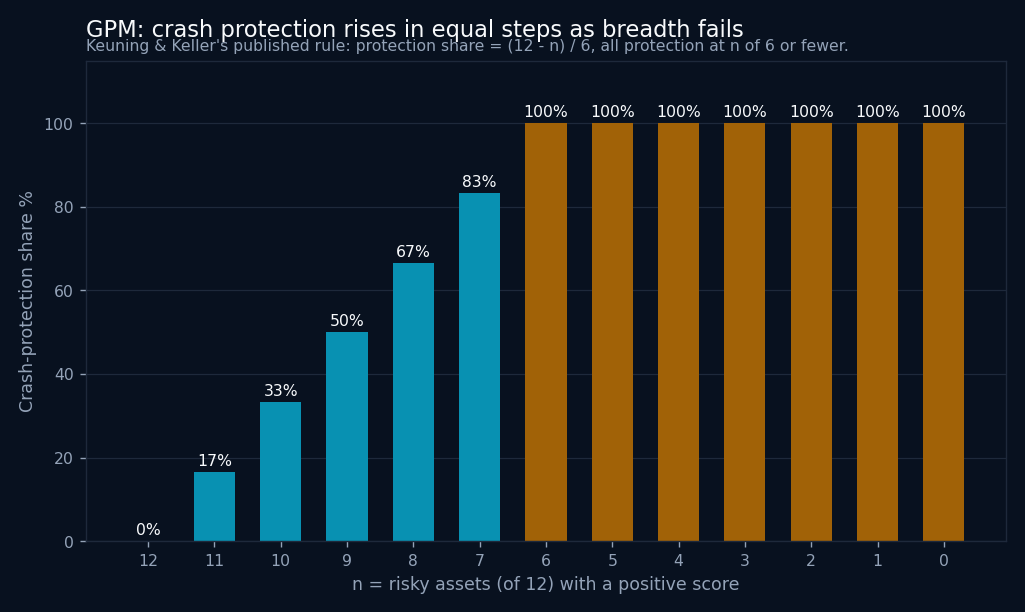
Generalized Protective Momentum looks like a ranking strategy until breadth weakens. It scores 12 risky assets, selects 3 leaders, and then asks a separate question: how many assets have a positive score at all? The fewer there are, the more of the portfolio goes to crash protection, in equal steps, until at 6 or fewer the whole portfolio is protected.
The current BestFolio card for the standard GPM implementation covers 41.8 years, from January 1985 through October 2026. It reports 10.57% annualized return, a 0.86 Sharpe ratio, 8.36% volatility, and a -15.13% maximum drawdown. The modest return and low volatility fit the strategy's intended role: protection and portfolio ballast rather than a standalone return engine.
Step 1: score the universe
GPM's universe is 12 risky assets: US large, tech-heavy and small-cap stocks (SPY, QQQ, IWM), Europe, Japan and emerging markets (VGK, EWJ, EEM), real estate (VNQ), commodities (DBC), gold (GLD), high-yield and investment-grade corporate bonds (HYG, LQD) and long Treasuries (TLT). Each asset's raw momentum is the average of its 1-month, 3-month, 6-month and 12-month total returns.
The score is then adjusted by how correlated the asset has been with the equal-weight mix of all 12 over the last 12 monthly returns: score = momentum x (1 - correlation). An asset with strong momentum and a lower correlation receives more credit than another leader moving in lockstep with everything else. Keuning and Keller's design is not only looking for what has risen. It is looking for leaders that add something different.
Step 2: count positive scores
Let n be the number of risky assets with a positive score. The crash-protection share is (12 - n) / 6: nothing when all 12 are positive, one sixth more for each asset that drops out, half at 9, and the whole portfolio at 6 or fewer. The rest is split equally among the 3 highest-scoring risky assets.
The protection itself is not fixed. GPM scores IEF and short-term Treasuries (SHV) the same way and holds whichever scores higher, so when rates are falling the protection can be intermediate Treasuries rather than cash.
This gives the strategy 2 defensive behaviors. Weakening breadth scales protection upward while the portfolio still owns leaders. Breadth at half the universe or below sends the whole portfolio to protection.
Why the breadth rule helps
Relative momentum always finds a winner. In a broad decline, the best-ranked risky asset can simply be the one losing least. The positivity count stops that ranking machine from turning a bad universe into a confident allocation.
The rule also makes the strategy auditable. There is no discretion about whether the backdrop feels dangerous. A reader can reproduce the 12 scores, count the positives, and know the next allocation.
Where it can still hurt
Every step is still a threshold: each asset that crosses zero moves a sixth of the portfolio. Suppose several assets sit just above or below zero. A small data revision or a different month-end close can change the count and move a sixth or a third of the portfolio between risk and protection. The steps are even, so there is no single cliff, but nearby months can still look more different than they are.
That raises practical questions for any implementation. Are the inputs adjusted for distributions? Is the score computed from official month-end closes? Does the backtest trade on information that was available at the time? Does a 1-day delay change the historical switches? GPM's published rule is precise enough to test those questions, which is an advantage, but the clean rule does not remove the timing risk.
How I would use it
GPM's 10.57% annualized return should not be compared with a concentrated equity strategy as if the 2 were substitutes. Its 8.36% volatility and -15.13% maximum drawdown show a different job. In a blended portfolio, the question is whether GPM's defensive switches and low-correlation leaders improve the total allocation.
I would also watch the months when breadth sits near the middle of the universe. A backtest summary can tell us the long-run effect of the rule. The switch log tells us whether the investor could follow it through a cluster of rapid moves between risk and protection.
The design's best idea is simple: do not confuse the highest-ranked asset with a healthy opportunity set. GPM turns that idea into a rule anyone can check.
Explore Generalized Protective Momentum.
Past performance does not guarantee future results. Backtested results are hypothetical and do not represent actual trading.